LeNet

Handwritten Digit Recognition with a Back-Propagation Network(NIPS1989)
[paper]

LeNet由2个卷积层和3个全连接层组成，每个卷积层之后有一个Sigmoid激活函数和一个AvgPool2d平均汇聚层，前两层全连接层之后也有一个Sigmoid激活函数。
具体模型架构如图：

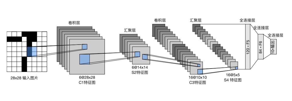
LeNet模型图

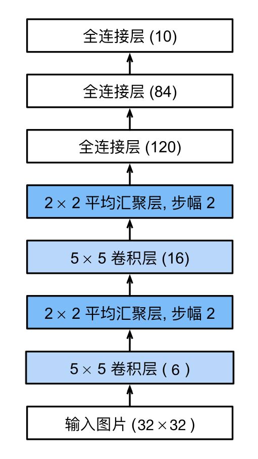
LeNet网络架构图

基于pytorch实现LeNet网络的模型搭建如下：

模型建立

import torch
import torch.nn as nn
import torch.nn.functional as F


class LeNet(nn.Module):
    def __init__(self, in_channels, num_classes):
        super(LeNet, self).__init__()
        """
        num_classes:分类的数量
        in_channels:原始图像通道数,灰度图像为1,彩色图像为3
        """
        self.num_classes = num_classes
        self.lenet = nn.Sequential(
            nn.Conv2d(in_channels, 6, kernel_size=5),  # (32 - 5) / 1 + 1 = 28   [3, 32, 32] -> [6, 28, 28]
            nn.Sigmoid(),
            # 也可用最大池化 
            nn.AvgPool2d(kernel_size=2, stride=2),  # 28 / 2 = 14   [6, 28, 28] -> [6, 14, 14]
            nn.Conv2d(6, 16, kernel_size=5),  # (14 - 5) / 1 + 1 = 10   [6, 14, 14] -> [16, 10, 10]
            nn.Sigmoid(),
            nn.AvgPool2d(kernel_size=2, stride=2), # 10 / 2 = 5   [16, 10, 10] -> [16, 5, 5]
            nn.Flatten(), # 展平
            nn.Linear(16 * 5 * 5, 120),
            nn.Sigmoid(),
            nn.Linear(120, 84),
            nn.Sigmoid(),
            nn.Linear(84, num_classes)) # 不需要使用激活函数，因为softmax激活函数被嵌入在交叉熵函数中

    def forward(self, x):
        output = self.lenet(x)
        # probas = F.softmax(output, dim=1)
        return output #, probas

模型检验

打印出各层的参数

num_classes = 10
in_channels = 3
X = torch.rand(size=(1, in_channels, 32, 32), dtype=torch.float32)
net = LeNet(in_channels, num_classes)
for layer in net.lenet:
  X = layer(X)
  print(layer.__class__.__name__,'output shape: \t',X.shape)

结果为：

Conv2d output shape: 	 torch.Size([1, 6, 28, 28])
Sigmoid output shape: 	 torch.Size([1, 6, 28, 28])
AvgPool2d output shape:  torch.Size([1, 6, 14, 14])
Conv2d output shape: 	 torch.Size([1, 16, 10, 10])
Sigmoid output shape: 	 torch.Size([1, 16, 10, 10])
AvgPool2d output shape:  torch.Size([1, 16, 5, 5])
Flatten output shape: 	 torch.Size([1, 400])
Linear output shape: 	 torch.Size([1, 120])
Sigmoid output shape: 	 torch.Size([1, 120])
Linear output shape: 	 torch.Size([1, 84])
Sigmoid output shape: 	 torch.Size([1, 84])
Linear output shape: 	 torch.Size([1, 10])

AlexNet

ImageNet Classification with Deep Convolutional Neural Networks(NIPS2012)
[paper]
AlexNet与LeNet网络架构基本相似，只是AlexNet更深，使用了8层卷积神经网络（5个卷积层，3个最大汇聚层），并且使用的激活函数不再是Sigmoid而是ReLU。

其具体网络架构如下:

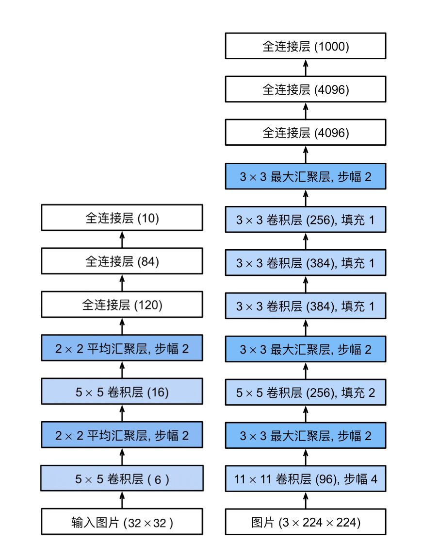
LeNet架构图（左）AlexNet架构图（右）

基于pytorch实现AlexNet网络的模型搭建如下：

模型建立

import torch
import torch.nn as nn
import torch.nn.functional as F


class AlexNet(nn.Module):
    def __init__(self, in_channels, num_classes):
        super(AlexNet, self).__init__()
        """
        num_classes:分类的数量
        in_channels:原始图像通道数,灰度图像为1,彩色图像为3
        """
        self.num_classes = num_classes
        self.lenet = nn.Sequential(
            nn.Conv2d(in_channels, 96, kernel_size=11, stride=4, padding=2),  # (224 - 11 + 4) / 4 + 1 = 55.25   [3, 224, 224] -> [96, 55, 55]
            nn.ReLU(),
            nn.MaxPool2d(kernel_size=3, stride=2),  # (55 + 2 - 3) / 2 = 27   [96, 55, 55] -> [96, 27, 27]
            nn.Conv2d(96, 256, kernel_size=5, padding=2),  # (27 - 5 + 4) / 1 + 1 = 27   [96, 27, 27] -> [256, 27, 27]
            nn.ReLU(),
            nn.MaxPool2d(kernel_size=3, stride=2), # (27 - 3 + 2) / 2 = 13   [256, 27, 27] -> [256, 13, 13]
            nn.Conv2d(256, 384, kernel_size=3, padding=1),  # (13 - 3 + 2) / 1 + 1 = 13   [256, 13, 13] -> [384, 13, 13]
            nn.ReLU(),
            nn.Conv2d(384, 384, kernel_size=3, padding=1),  # (13 - 3 + 2) / 1 + 1 = 13   [384, 13, 13] -> [384, 13, 13]
            nn.ReLU(),
            nn.Conv2d(384, 256, kernel_size=3, padding=1),  # (13 - 3 + 2) / 1 + 1 = 13   [384, 13, 13] -> [256, 13, 13]
            nn.ReLU(),
            nn.MaxPool2d(kernel_size=3, stride=2), # (13 - 3 + 2) / 2 = 6   [256, 13, 13] -> [256, 6, 6]
            nn.Flatten(), # 展平
            nn.Linear(256 * 6 * 6, 4096),
            nn.ReLU(),
            nn.Dropout(p=0.5),
            nn.Linear(4096, 4096),
            nn.ReLU(),
            nn.Dropout(p=0.5),
            nn.Linear(4096, num_classes)) # 不需要使用激活函数，因为softmax激活函数被嵌入在交叉熵函数中

    def forward(self, x):
        output = self.lenet(x)
        # probas = F.softmax(output, dim=1)
        return output #, probas

在第一次卷积操作时，不能完全遍历整个图像，应该在左、上添两列零，右、下添一列零能完全遍历；使用padding=2填充，在操作过程中会自动省去多余数据，故影响不大。

模型检验

打印出各层的参数

num_classes = 1000
in_channels = 3
X = torch.rand(size=(1, in_channels, 224, 224), dtype=torch.float32)
net = AlexNet(in_channels, num_classes)
for layer in net.lenet:
  X = layer(X)
  print(layer.__class__.__name__,'output shape: \t',X.shape)

结果为：

Conv2d output shape: 	 torch.Size([1, 96, 55, 55])
ReLU output shape: 	 torch.Size([1, 96, 55, 55])
MaxPool2d output shape:  torch.Size([1, 96, 27, 27])
Conv2d output shape: 	 torch.Size([1, 256, 27, 27])
ReLU output shape: 	 torch.Size([1, 256, 27, 27])
MaxPool2d output shape:  torch.Size([1, 256, 13, 13])
Conv2d output shape: 	 torch.Size([1, 384, 13, 13])
ReLU output shape: 	 torch.Size([1, 384, 13, 13])
Conv2d output shape: 	 torch.Size([1, 384, 13, 13])
ReLU output shape: 	 torch.Size([1, 384, 13, 13])
Conv2d output shape: 	 torch.Size([1, 256, 13, 13])
ReLU output shape: 	 torch.Size([1, 256, 13, 13])
MaxPool2d output shape:  torch.Size([1, 256, 6, 6])
Flatten output shape: 	 torch.Size([1, 9216])
Linear output shape: 	 torch.Size([1, 4096])
ReLU output shape: 	 torch.Size([1, 4096])
Dropout output shape: 	 torch.Size([1, 4096])
Linear output shape: 	 torch.Size([1, 4096])
ReLU output shape: 	 torch.Size([1, 4096])
Dropout output shape: 	 torch.Size([1, 4096])
Linear output shape: 	 torch.Size([1, 1000])

AlexNet与LeNet不同

网络更深，使用8层网络进行训练
激活函数改进，使用ReLU替代Sigmoid，减少梯度消失现象
池化层采用Maxpool2d代替Avgpool2d，避免平均池化的模糊化效果，并且在池化的时候让步长比池化核的尺寸小，这样池化层的输出之间会有重叠和覆盖，提升了特征的丰富性
在全连接层处使用Dropout丢弃法，防止过拟合
在数据增强部分使用crop、PCA、加高斯噪声等
提出了LRN层，对局部神经元的活动创建竞争机制，使得其中响应比较大的值变得相对更大，并抑制其他反馈较小的神经元，增强了模型的泛化能力。

NiN

Network in Network(ICLR2014)
[paper]

NiN块

NiN块以⼀个普通卷积层开始，后⾯是两个$1 \times 1$的卷积层。这两个$1 \times 1$卷积层充当带有ReLU激活函数的逐像素全连接层。第⼀层的卷积窗口形状通常由用户设置，随后的卷积窗口形状固定为$1 \times 1$。

所以NiN块可以定义为：

import torch
import torch.nn as nn

def nin(in_channels, out_channels, kernel_size, strides, padding):
    nin_block = nn.Sequential(
        nn.Conv2d(in_channels, out_channels, kernel_size, strides, padding),
        nn.ReLU(),
        nn.Conv2d(out_channels, out_channels, kernel_size=1),
        nn.ReLU(),
        nn.Conv2d(out_channels, out_channels, kernel_size=1),
        nn.ReLU())
    return nin_block

NiN块和NiN的架构如下：

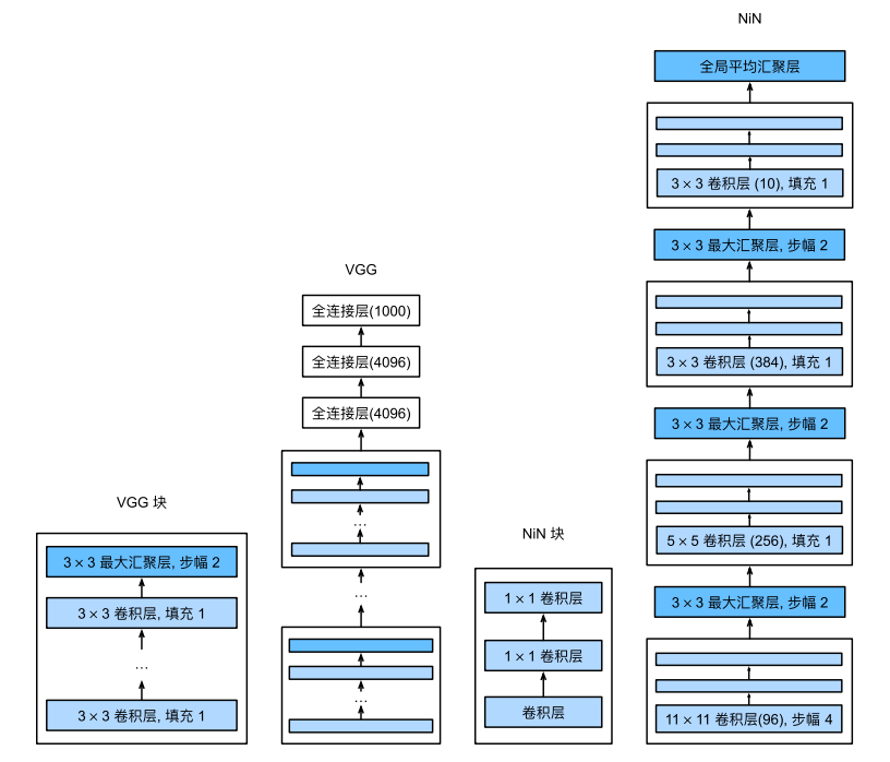
VGG块及其网络架构（左）NiN块及其网络架构（右）

基于pytorch实现NiN网络的模型搭建如下：

in_channels = 1
num_classes = 10

nin_net = nn.Sequential(
    nin(in_channels, 96, kernel_size=11, strides=4, padding=0),
    nn.MaxPool2d(kernel_size=3, stride=2),
    nin(96, 256, kernel_size=5, strides=1, padding=2),
    nn.MaxPool2d(kernel_size=3, stride=2),
    nin(256, 384, kernel_size=3, strides=1, padding=1),
    nn.MaxPool2d(kernel_size=3, stride=2),
    nn.Dropout(p=0.5),
    nin(384, num_classes, kernel_size=3, strides=1, padding=1),
    nn.AdaptiveAvgPool2d((1, 1)),
    nn.Flatten())

模型检验

X = torch.randn(size=(in_channels, 1, 224, 224))
net = nin_net
for layer in net:
    X = layer(X)
    print(layer.__class__.__name__,'output shape: \t',X.shape)

结果为：

Sequential output shape: 	 torch.Size([1, 96, 54, 54])
MaxPool2d output shape: 	 torch.Size([1, 96, 26, 26])
Sequential output shape: 	 torch.Size([1, 256, 26, 26])
MaxPool2d output shape: 	 torch.Size([1, 256, 12, 12])
Sequential output shape: 	 torch.Size([1, 384, 12, 12])
MaxPool2d output shape: 	 torch.Size([1, 384, 5, 5])
Dropout output shape: 	         torch.Size([1, 384, 5, 5])
Sequential output shape: 	 torch.Size([1, 10, 5, 5])
AdaptiveAvgPool2d output shape:  torch.Size([1, 10, 1, 1])
Flatten output shape: 	         torch.Size([1, 10])

NiN结构包括3个mplconv层和一个全局平均池化层(GAP)，3个mplconv层分别使用了$11\times 11$、$5\times 5$和$3\times 3$的卷积核，卷积操作后再接两个全连接层，每个NiN块后有一个最大池化层，核为$3\times 3$，步幅为2，此池化层有GAP不同。

NiN和AlexNet之间的一个显著区别是NiN完全取消了全连接层。NiN使用的是一个NiN块，其输出通道数等于标签类别的数量。最后放一个全局平均汇聚层，生成一个对数几率。

NiN设计的一个优点是，它显著减少了模型所需参数的数量，但是有时会增加训练模型的时间。

VGG

Very Deep Convolutional Networks for Large-Scale Image Recognition(ICLR2015)
[paper]

VGG块

VGG块与经典卷积神经网络一样，由一系列卷积层、激活函数和汇聚层组成，每一个VGG块只有卷积层个数、输入通道数和输出通道数不一样，所以，一个VGG块可以定义为：

import torch
import torch.nn as nn


def vgg_block(num_convs, in_channels, out_channels):
    layers = []
    for _ in range(num_convs):
        layers.append(nn.Conv2d(in_channels, out_channels, kernel_size=3, padding=1))
        layers.append(nn.ReLU())
        in_channels = out_channels
    layers.append(nn.MaxPool2d(kernel_size=2, stride=2))
    return nn.Sequential(*layers)

VGG神经网络就是由多个不同卷积层个数、输入通道数和输出通道数的VGG块共同组成卷积层，最后再连接3个全连接层组成整个神经网络，其架构如图所示：

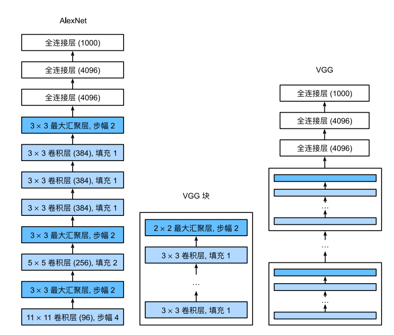
AlexNet架构图（左）VGG块（中） VGG架构图（右）

基于pytorch实现VGG网络的模型搭建如下：

模型建立

def vggnet(conv, num_classes):
    conv_layers = []
    in_channels = 1
    # 调用VGG块定义卷积层模块
    for (num_convs, out_channels) in conv:
        conv_layers.append(vgg_block(num_convs, in_channels, out_channels))
        in_channels = out_channels

    net_vgg = nn.Sequential(
        *conv_layers,
        nn.Flatten(),
        nn.Linear(out_channels * 7 * 7, 4096),
        nn.ReLU(),
        nn.Dropout(p=0.5),
        nn.Linear(4096, 4096),
        nn.ReLU(),
        nn.Dropout(p=0.5),
        nn.Linear(4096, num_classes),
        )
    return net_vgg

定义不同的vgg块：

conv11 = ((1, 64), (1, 128), (2, 256), (2, 512), (2, 512)) # VGG_11
conv13 = ((2, 64), (2, 128), (2, 256), (2, 512), (2, 512)) # VGG_13
conv16 = ((2, 64), (2, 128), (3, 256), (3, 512), (3, 512)) # VGG_16
conv19 = ((2, 64), (2, 128), (4, 256), (4, 512), (4, 512)) # VGG_19
num_classes = 1000

net = vggnet(conv16, num_classes)

模型检验

构建一个高度和宽度为224的单通道数据样本，观察每个层输出的形状

X = torch.randn(size=(1, 1, 224, 224))
for layer in net:
    X = layer(X)
    print(layer.__class__.__name__,'output shape: \t',X.shape)

结果为：

Sequential output shape:   torch.Size([1, 64, 112, 112])
Sequential output shape:   torch.Size([1, 128, 56, 56])
Sequential output shape:   torch.Size([1, 256, 28, 28])
Sequential output shape:   torch.Size([1, 512, 14, 14])
Sequential output shape:   torch.Size([1, 512, 7, 7])
Flatten output shape: 	   torch.Size([1, 25088])
Linear output shape: 	   torch.Size([1, 4096])
ReLU output shape: 	   torch.Size([1, 4096])
Dropout output shape:  	   torch.Size([1, 4096])
Linear output shape: 	   torch.Size([1, 4096])
ReLU output shape:  	   torch.Size([1, 4096])
Dropout output shape: 	   torch.Size([1, 4096])
Linear output shape: 	   torch.Size([1, 1000])

VGG采用的都是$3 \times 3$的卷积，在取得相同的感受野的情况下，计算量小了很多；多层小卷积可以引入更多的非线性，从而使模型的拟合能力更强；方便优化卷积计算。

在经过每一个VGG块后，图像高宽减半，通道数增加。从上面四个VGG模型可以看到，无论是VGG多少，都有5个VGG模块，而且这五个模块仅仅是num_convs不一样，每一个模块对应的out_channels是一样的。

由于VGG所含有的卷积层更多，网络更深，所以计算量比AlexNet更大，计算也慢很多。

GoogLeNet

Going Deeper with Convolutions(CVPR2015)
[paper]

Inception块

在GoogLeNet中，最新的改进是新加入了基本卷积块Inception块，网络架构开始出现分支，并不是一条线连到底。

Inception块有四条并行分支路径，前三条路径使用的卷积核大小为$1\times1$、$3\times3$和$5\times5$，从不同空间大小中提取信息。中间的两条路径在输入上执行$1\times1$卷积，以减少通道数，从而降低模型的复杂性。第四条路径使用$3\times3$最大汇聚层，然后使用$1\times1$卷积层来改变通道数。

这四条路径都使用合适的填充来确保输入与输出的高和宽一致，这样才能将每条线路的输出在通道维度上连结，并构成Inception块的输出。在Inception块中，通常调整的超参数是每层输出通道数。

Inception的架构为：

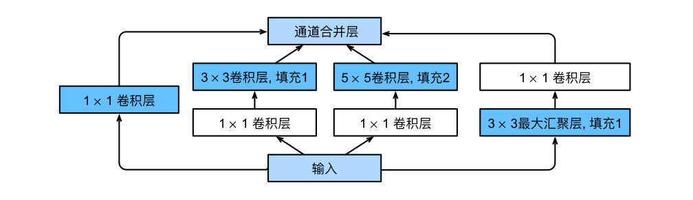
Inception块架构

Inception块定义为：

import torch
import torch.nn as nn

class Inception(nn.Module):
    def __init__(self, in_channels, c1, c2, c3, c4, **kwargs):
        super(Inception, self).__init__(**kwargs)
        
        # 支路一
        self.b1 = nn.Sequential(
            nn.Conv2d(in_channels, c1, kernel_size=1),
            nn.ReLU())
        # 支路二
        self.b2 = nn.Sequential(
            nn.Conv2d(in_channels, c2[0], kernel_size=1),
            nn.ReLU(),
            nn.Conv2d(c2[0], c2[1], kernel_size=3, padding=1),
            nn.ReLU())
        # 支路三
        self.b3 = nn.Sequential(
            nn.Conv2d(in_channels, c3[0], kernel_size=1),
            nn.ReLU(),
            nn.Conv2d(c3[0], c3[1], kernel_size=5, padding=2),
            nn.ReLU())
        # 支路四
        self.b4 = nn.Sequential(
            nn.MaxPool2d(kernel_size=3, stride=1, padding=1),
            nn.Conv2d(in_channels, c4, kernel_size=1),
            nn.ReLU())
        
    def forward(self, x):
        output1 = self.b1(x)
        output2 = self.b2(x)
        output3 = self.b3(x)
        output4 = self.b4(x)

        outputs = [output1, output2, output3, output4]
        return torch.cat(outputs, 1)

GoogLeNet模型

GoogLeNet是由一些基本的卷积核和9个Inception块进行卷积操作后连接一个全局平均汇聚层，最后再连接一个全连接层完成输出。

GoogLeNet的网络框架为：

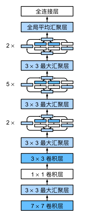
GoogLeNet的网络框架

基于pytorch实现GoogLeNet网络的模型搭建如下：

class GoogLeNet(nn.Module):
    def __init__(self, in_channels, num_classes):
        super(GoogLeNet, self).__init__()

        self.m1 = nn.Sequential(
            nn.Conv2d(in_channels, 64, kernel_size=7, stride=2, padding=3),
            nn.ReLU(),
            nn.MaxPool2d(kernel_size=3, stride=2, padding=1))
        
        self.m2 = nn.Sequential(
            nn.Conv2d(64, 64, kernel_size=1),
            nn.ReLU(),
            nn.Conv2d(64, 192, kernel_size=3, padding=1),
            nn.ReLU(),
            nn.MaxPool2d(kernel_size=3, stride=2, padding=1))
        
        self.m3 = nn.Sequential(
            Inception(192, 64, (96, 128), (16, 32), 32),
            Inception(256, 128, (128, 192), (32, 96), 64),
            nn.MaxPool2d(kernel_size=3, stride=2, padding=1))
        
        self.m4 = nn.Sequential(
            Inception(480, 192, (96, 208), (16, 48), 64),
            Inception(512, 160, (112, 224), (24, 64), 64),
            Inception(512, 128, (128, 256), (24, 64), 64),
            Inception(512, 112, (144, 288), (32, 64), 64),
            Inception(528, 256, (160, 320), (32, 128), 128),
            nn.MaxPool2d(kernel_size=3, stride=2, padding=1))
        
        self.m5 = nn.Sequential(
            Inception(832, 256, (160, 320), (32, 128), 128),
            Inception(832, 384, (192, 384), (48, 128), 128),
            nn.AdaptiveAvgPool2d((1, 1)),
            nn.Dropout(p=0.5),
            nn.Flatten())
        
        self.googlenet = nn.Sequential(self.m1, self.m2, self.m3, self.m4, self.m5, nn.Linear(1024, num_classes))
    
    def forward(self, x):
        x = self.googlenet(x)
        return x

模型检验

构建一个高度和宽度为224的单通道数据样本，观察每个层输出的形状

in_channels = 3
num_classes = 10
X = torch.randn(size=(1, in_channels, 224, 224))
net = GoogLeNet(in_channels, num_classes)
print(net(X))
for layer in net.googlenet:
    X = layer(X)
    print(layer.__class__.__name__,'output shape: \t',X.shape)

结果为：

tensor([[ 0.0278,  0.0170,  0.0201,  0.0070,  0.0244,  0.0257,  0.0028, -0.0330,
         -0.0201, -0.0199]], grad_fn=<AddmmBackward0>)
Sequential output shape: 	 torch.Size([1, 64, 56, 56])
Sequential output shape: 	 torch.Size([1, 192, 28, 28])
Sequential output shape: 	 torch.Size([1, 480, 14, 14])
Sequential output shape: 	 torch.Size([1, 832, 7, 7])
Sequential output shape: 	 torch.Size([1, 1024])
Linear output shape: 	         torch.Size([1, 10])

Inception块相当于⼀个有4条路径的⼦⽹络。它通过不同窗口形状的卷积层和最⼤汇聚层来并⾏抽取信息，并使⽤$1\times1$卷积层减少每像素级别上的通道维数从而降低模型复杂度。
GoogLeNet将多个设计精细的Inception块与其他层（卷积层、全连接层）串联起来。其中Inception块的通道数分配之⽐是在ImageNet数据集上通过⼤量的实验得来的。
GoogLeNet和它的后继者们⼀度是ImageNet上最有效的模型之⼀：它以较低的计算复杂度提供了类似的测试精度。

另外：GoogLeNet还在第四个大模块的第1个(Inception4a)和第4个模块(Inception4d)后添加辅助分类器：其架构如图:

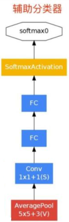
GoogLeNet的辅助分类器的网络框架

实现如下：

class Assisant(nn.Module):
    def __init__(self, in_channels, num_classes):
        super(Assisant, self).__init__()
        self.feature = nn.Sequential(
            nn.AvgPool2d(kernel_size=5, stride=3),
            nn.Conv2d(in_channels, 128, kernel_size=1),
            nn.ReLU(),
            nn.Flatten(),
            nn.Dropout(p=0.5),
            nn.Linear(2048, 1024),
            nn.ReLU(),
            nn.Dropout(p=0.5),
            nn.Linear(1024, num_classes))

        self.fc1 = nn.Linear(2048, 1024)
        self.fc2 = nn.Linear(1024, num_classes)

    def forward(self, x):
        x = self.feature(x)
        return x

辅助分类器仅在训练时使用，将3个分类器的损失函数加权求和，以缓解梯度消失现象。

Inception-v2

Batch Normalization: Accelerating Deep Network Training by Reducing Internal Covariate Shift(CVPR2016)
[papr]

使用Batch Normalization，将输出归一化为N(0,1),可以采用较大的学习速率，加快收敛，且BN具有正则效应，不需要太依赖dropout，减少过拟合。
卷积分解，$5 \times 5$的卷积分解为两个$3 \times 3$的卷积，使网络更深，参数更少。

Inception-v3

Rethinking the Inception Architecture for Computer Vision
[paper]

非对称分解卷积，将$n \times n$的卷积分解为两个$n \times 1$和$1 \times n$的卷积，使网络更深，参数更少。
设计了一个并行双分支的结构Grid Size Reduction来取代max pooling，边卷积边池化，最后再叠加，减少信息损失的同时减小参数量。
辅助分类器采用BatchNorm

四大设计原则：

在浅层不要过度降维或收缩特征
特征越多，收敛越快。
大卷积核之前用1 * 1卷积降维，信息不丢失
均衡网络中的深度和宽度

Inception-v4

Inception-v4, Inception-ResNet and the Impact of Residual Connections on Learning(AAAI2017)
[paper]

引入了ResNet，使训练加速，性能提升。卷积时先加入1 * 1的卷积降维减少运算量
当滤波器的数目过大（>1000）时，训练很不稳定，提出了缩小因子解决残差块的不稳定现象(在inception之后先乘以缩小因子，然后和恒等映射相加)

Xception

Xception: Deep Learning with Depthwise Separable Convolutions(CVPR2017)
[paper]

在Inception-v3的基础上提出，基本思想是通道分离式卷积。模型参数稍微减少，但是精度更高。Xception卷积的时候要将通道的卷积与空间的卷积进行分离，先做1×1卷积再做3×3卷积，即先将通道合并，再进行空间卷积。
Xception使用了激活函数Relu

ResNet

初始ResNet

Deep Residual Learning for Image Recognition(CVPR2016)
[paper]

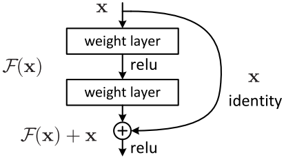
残差块

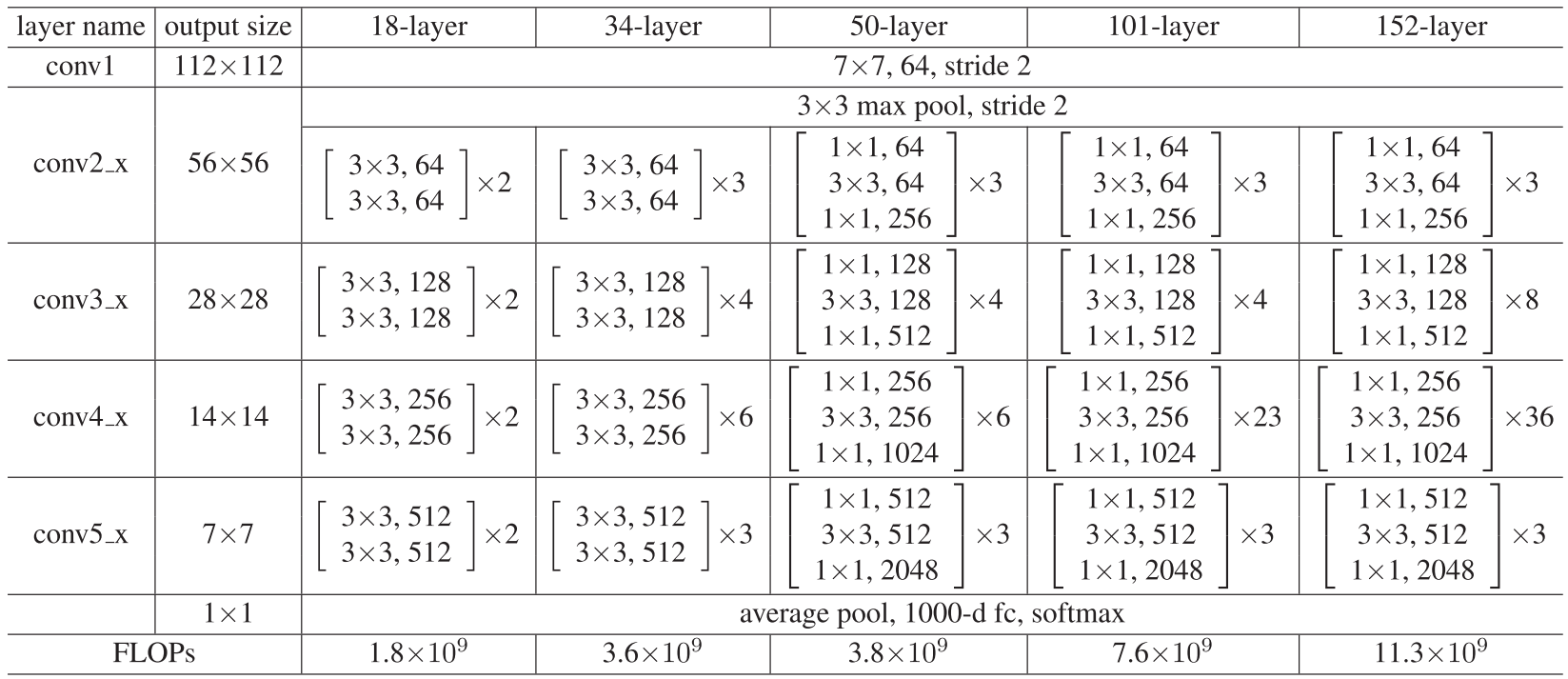
由于更深的网络极易导致梯度弥散，从而导致网络无法收敛。经测试，20层以上会随着层数增加收敛效果越来越差，ResNet 的核心思想则是采用了identity shortcut connection，构建了一个个残差块。残差块有两种连接方式，一种是input和output的size一样，直接相连；另一种是input和output的size不一样，要先通过一个卷积层conv去完成resize再进行相连。 ResNet有以下几种：ResNet18、ResNet34、ResNet50、ResNet101、ResNet152

ResNet网络参数表

ResNet变种

ResNeXt

Aggregated Residual Transformations for Deep Neural Networks(CVPR2017)
[paper] [code]
一般来说增加网络表达能力的途径有三种：

增加网络深度，如从AlexNet到ResNet，但是实验结果表明由网络深度带来的提升越来越小
增加网络模块的宽度，但是宽度的增加必然带来指数级的参数规模提升，也非主流CNN设计
改善CNN网络结构设计，如Inception系列和ResNeXt等。且实验发现增加Cardinatity即一个block中所具有的相同分支的数目可以更好的提升模型表达能力

ResNeXt同样堆叠block，参考类似Inception的方式，使得ResNet更宽，每个block中每一个path都是相同的。

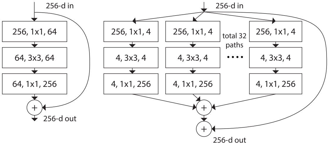
残差块

DenseNet

Densely Connected Convolutional Networks(CVPR2017)
[paper] [code]
DenseNet 脱离了加深网络层数(ResNet)和加宽网络结构(Inception)来提升网络性能的定式思维，从特征的角度考虑，通过特征重用和旁路(Bypass)设置，既大幅度减少了网络的参数量，又在一定程度上缓解了梯度消失问题的产生。

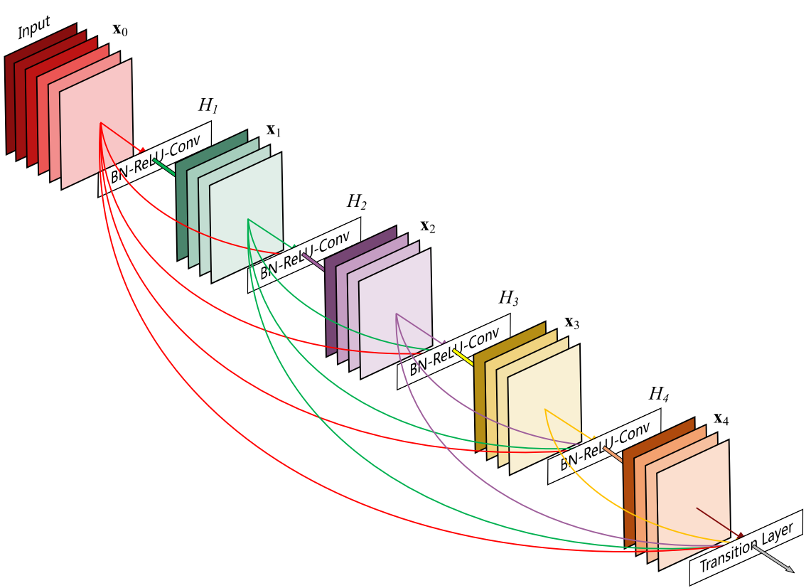
DenseNet block

第$i$层的输入不仅与$i-1$层的输出有关，还与之前所有层的输出都有关。
$X_l=H_l([X_0,X_1,…,X_l-1])$，其中[]表示concatenation拼接操作，将前面层的输出feature map按通道组合在一起。

由于需要对不同层的feature map进行cat操作，所以需要不同层的feature map保持相同的size，这就限制了网络中Down sampling的实现。所以同样采用不同的Denseblock，同一个Denseblock中feature size相同，在不同Denseblock之间进行Down sampling。

每一个Denseblock中提出了Growth rate的概念，即每个网络层输出的特征图数量K，决定着每一层需要给全局状态更新的信息的多少。

DenseNet接受较少的K，但由于不同层feature map之间由cat操作组合在一起，最终仍导致channel较大而成为网络的负担。所以使用1×1 Conv(Bottleneck)作为特征降维的方法来降低channel数量。
优点：

减轻了梯度消失
加强了feature的传递
更有效地利用了feature
一定程度上较少了参数数量

DenseNet有以下几种：DenseNet-121(k=32)、DenseNet-169(k=32)、DenseNet-201(k=32)、DenseNet-161(k=48)

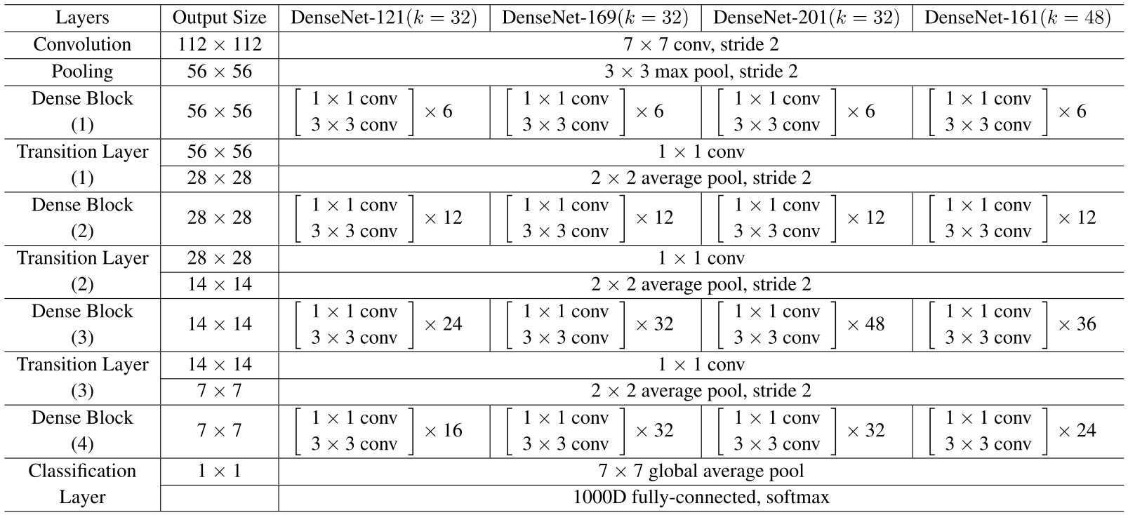
DenseNet网络参数表

Res2Net

Res2Net: A New Multi-scale Backbone Architecture(PAMI2021)
[paper] [code]

ResNeSt

ResNeSt: Split-Attention Networks(CVPR2022)
[paper] [code]

SqueezeNet

SqueezeNet: AlexNet-level accuracy with 50x fewer parameters and <0.5MB model size(ICLR)
[paper]
轻量化网络的实现：

优化网络结构，如ShuffleNet
减少模型参数，如SqueezeNet
优化卷积操作，如MobileNet改变卷积操作、Winograd从算法角度优化卷积
提出FC，如SqueezeNet、LightCNN

核心是提出fire module，分为两个部分squeeze和expend

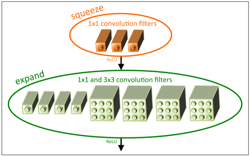
fire module架构图

squeeze层是一组连续的$1 \times 1$卷积，expand层用一组连续的$1 \times 1$和一组连续的$3 \times 3$分别卷积，然后concatenation。SqueezeNet参数是Alexnet的1/50，经过压缩之后是1/510，但是准确率相当。

MobileNet

V1

MobileNets: Efficient Convolutional Neural Networks for Mobile Vision Applications(CVPR2017)
[paper] [code]

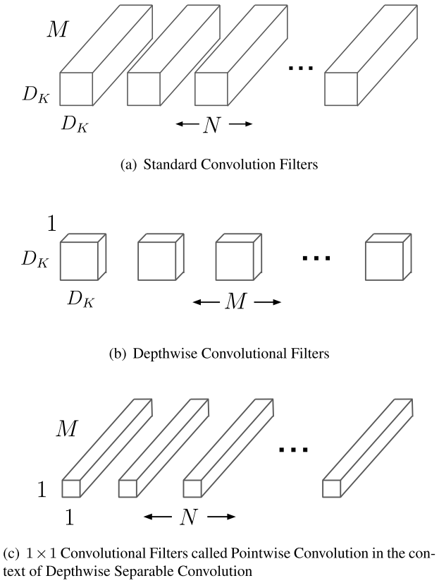
深度可分离卷积架构图

提出深度可分离网络(Depthwise Separable Convolution)；引入两个参数，宽度超参数$\alpha$控制输入输出通道数；分辨率超参数$\beta$控制图像（特征图）分辨率。

Depthwise Separable Convolution由两部分组成：深度卷积(DW)和逐点卷积(PW)。
DW卷积中每个卷积核的channel都为1，一个卷积核只有一个通道，负责一个通道，卷积核个数=输入特征channel数=输出特征channel数
PW是卷积核大小为1的普通卷积，分别与DW输出的特征图做卷积操作，将上一步的特征图在通道方向进行扩展
DW+PW共同实现了以往普通卷积的功能，但参数量减少到原来的1/9~1/8

V2

MobileNetV2: Inverted Residuals and Linear Bottlenecks(CVPR2018)
[paper] [code]

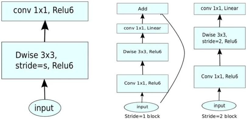
Inverted Residuals

深度卷积本身没有改变通道的能力，来的是多少通道输出就是多少通道。如果来的通道很少的话，DW深度卷积只能在低维度上工作，这样效果并不会很好，所以需要“扩张”通道。先在DW深度卷积之前使用PW卷积进行升维（升维倍数为t，t=6），再在一个更高维的空间中进行卷积操作来提取特征。先升维再卷积再降维，引入shortcut结构复用特征，此结构与残差块的先降维再卷积再升维刚好相反，所以叫做逆残差块。
最后的ReLU层改为Linear层，这是因为ReLU这种激活函数能有效增加特征的非线性表达，但是仅限于高维空间中，如果降低维度，再使用ReLU则会破坏特征，所以改用Linear层。
先进行$1 \times 1$卷积升维，再进行$3 \times 3$深度卷积提取特征，再通过Linear的逐点卷积降维。只有在步长为1时，将input与output相加，形成残差结构。步长为2时，因为input与output的尺寸不符，不添加shortcut结构，其余均一致。

V3

Searching for MobileNetV3(ICCV2019)
[paper] [code]

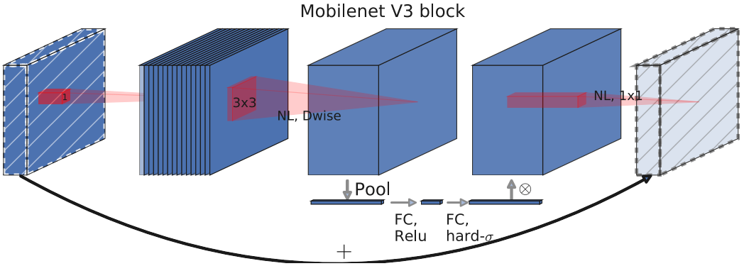
V3 block

保留V1中的深度可分离卷积和V2中的逆残差模块
引入SE结构的轻量级注意力模型，使用全局信息（全局池化）来增强有用的信息，同时抑制无用的信息（Sigmoid函数输出0、1），通过压缩、激励，调整每个通道的权重
用h-swish激活函数代替swish函数，减少运算量，提高性能
互补搜索技术组合：由资源受限的NAS执行模块集搜索，NetAdapt执行局部搜索（层级搜索Layer-wise Search）。
在V2的最后几层，把average pooling提前，提前把feature的size从$7 \times 7$降到了$1 \times 1$，延时减小了，但是精度却几乎没有降低。

ShuffleNet

V1

ShuffleNet: An Extremely Efficient Convolutional Neural Network for Mobile Devices(CVPR2018)
[paper]

提出逐点群卷积(pointwise group convolution)
提出通道混洗(channel shuffle)

V2

ShuffleNet V2: Practical Guidelines for Efficient CNN Architecture Design(ECCV2018)
[paper]

输入通道数与输出通道数保持相等可以最小化内存访问成本
分组卷积中使用过多的分组会增加内存访问成本
网络结构太复杂（分支和基本单元过多）会降低网络的并行程度
element-wise的操作消耗也不可忽略

EfficientNet

EfficientNet: Rethinking Model Scaling for Convolutional Neural Networks(ICML2019)
[paper] [code]
用NAS（Neural Architecture Search）技术来搜索网络的图像输入分辨率r，网络的深度depth以及channel的宽度width三个参数的合理化配置

SENet

Squeeze-and-Excitation Networks(CVPR2018)
[paper]
SE Block主要有三步，分别是Squeeze，Excitation和Scale(Reweight)。

Squeeze：使用global average pooling将每个二维的特征通道变成一个实数，使其某种程度上具有全局的感受野
Excitation：通过参数w来为每个特征通道生成权重，其中参数w被学习用来显式地建模特征通道间的相关性。两个FC层，先降维至1/16，再升维回原维度，然后通过一个Sigmoid的门获得0~1之间归一化的权重
Scale(Reweight)：将归一化后的权重通过乘法逐通道加权到每个通道的特征上，完成在通道维度上的对原始特征的重标定。

SKNet

Selective Kernel Networks(CVPR2019)
[paper]
提出了一种动态选择机制，允许每个神经元根据输入信息的多个尺度自适应地调整其感受野大小。设计了一个名为Selective Kernel(SK)单元的构建块，其中使用由这些分支中的信息引导的softmax attention来融合具有不同卷积核大小的多个分支。对这些分支的不同关注产生了融合层中神经元的有效感受野的不同大小。多个SK单元被堆叠到称为Selective Kernel(SKNets)的深度网络中。